Keep one clock at three real waterfronts. Reveal which water level rises next, build a tide from repeating rhythms, and discover why the Moon does not give every coast the same pattern.
Enable JavaScript to change the conditions and run the interactive experiment.
Understand it
Make a prediction at two piers
Start with Boston and Pensacola at the same clock time. Which will rise next? Reveal the following record. On June 1, 2024 from 00:00 to 01:00 UTC, Boston falls from 2.838 to 2.328 meters while Pensacola rises from 0.514 to 0.523 meters. Those are real station values, each above its own local reference. The monitoring scene makes the numbers visible; it is not a film of that day.
A shared pull, different responses
The Moon attracts Earth and its water. Because its pull differs across Earth, there is a small tide-generating difference. The Sun contributes too. Water then responds through connected oceans, shelves and bays. Coastlines, depth, friction and rotation help shape the local timing and size of the tide. A drawing of two ocean bulges cannot tell you the level at every pier.
Give the repeating pieces their names
A tide curve can be represented by repeating components called tidal constituents. Our four rhythm cards are M2, S2, K1 and O1. Add or remove one and inspect its contribution at the shared clock time. They are mathematical pieces of one explanation, not separate layers of water. A component with a larger amplitude contributes a larger oscillation; shifting its phase changes timing.
Read three kinds of evidence
Our four-rhythm curve is an authored approximation fitted to June NOAA predictions. NOAA’s fuller prediction is a separate product. The station’s recorded water level is another. A mismatch between our approximation and NOAA shows what the small model leaves out. A mismatch between observation and NOAA can have several causes; the gap alone does not tell you which.
Keep the sea; change its coordinate
Mean Lower Low Water, or MLLW, is a local reference elevation. It is not the seafloor or an empty ocean. Change Boston’s reference to Mean Sea Level, MSL, and the opening 2.838-meter reading becomes 1.252 meters. The same waterline gets a different number. Switching to feet also changes the label, not the sea.
Look beyond a single day
Boston’s selected record is dominated by a twice-per-lunar-day rhythm. San Diego has a mixed pattern, including unequal successive highs and lows. Pensacola has strong daily components. These descriptions summarize behavior; they do not demand an exact high/low count inside every midnight-to-midnight window. Follow the dated curve before assigning a pattern.
Look closer at the science
Subtract a shared acceleration
In an Earth-centered translating, nonrotating frame, let μ be the distant body’s gravitational parameter, D its position from Earth’s center and r a surface marker’s position. The differential acceleration is aₜ(r)=μ[(D−r)/|D−r|³−D/|D|³]. We subtract the distant body’s acceleration at Earth’s center—not Earth’s own gravity. Both original lunar attractions point toward the Moon. The far-side difference points outward relative to Earth’s center because that side is attracted less strongly.
An arrow is not a solved ocean
For unit surface normal n=r/|r|, the radial part is (aₜ·n)n and the tangential part is aₜ−(aₜ·n)n. Tangential forcing helps redistribute water. Our static force lens does not solve ocean motion, friction, the Coriolis effect, continents, elasticity or loading. Its exaggerated arrows are acceleration directions and magnitudes, not predicted water heights or literal paths traveled by water.
Near and far are not exactly equal
With the source along +x, Earth radius 6,371 km and Moon distance 384,400 km, the exact near-side differential x acceleration is about +1.128×10⁻⁶ m/s²; the far-side value is about −1.073×10⁻⁶ m/s². The unequal magnitudes are a finite-distance result. These distances define an illustrative static geometry, not a dated ephemeris. Lunar μ comes from JPL DE440, with km³/s² converted to m³/s².
Why inverse cube appears
For Earth’s radius small compared with the distance D, the leading term is aₜ≈(μ/D³)[3(nD·r)nD−r], where nD points toward the source. A distance of 0.9 times the reference gives leading strength 1/0.9³≈1.3717 times as large. This is a differential-strength approximation; whole point-mass attraction instead scales as inverse square. Exact surface-vector ratios differ slightly. Neither factor multiplies the historical station records.
Four frequencies, local fingerprints
The source speeds are M2 28.984104°/hour, S2 30°/hour, K1 15.041069°/hour and O1 13.943035°/hour. Period equals 360° divided by speed: about 12.4206, 12, 23.9345 and 25.8193 hours. M2 is principal lunar semidiurnal; S2 is principal solar semidiurnal; K1 is lunisolar diurnal; O1 is principal lunar diurnal. K1 is not a Moon-only switch. Different fitted amplitudes and phases give the three stations different curves.
Exactly what our fit means
Let t be hours after June 1, 2024 00:00 UTC. Our model is h₄(t)=b₀+Σ[cⱼ cos(ωⱼt)+sⱼ sin(ωⱼt)], where ωⱼ is source speed times π/180 radians per hour. Nine coefficients—one mean offset and four cosine/sine pairs—were fitted by least squares to 720 June hourly NOAA predictions at each station. These coefficients are authored short-window fits, not new NOAA harmonic constants, observations or a complete hydrodynamic model.
Phase changes timing, not amplitude
Each fitted pair can also be written A cos(ωt−φ), with A=√(c²+s²) and φ=atan2(s,c). Adding positive lag δ gives A cos(ωt−φ−δ); a +90° lag moves the corresponding peak later by one-quarter period. This is a mathematical change to one modeled component. It does not physically move a harbor or determine what an altered coastline would do.
Why published phase constants need more context
NOAA’s fuller harmonic equation includes a mean level, amplitudes, time-varying amplitude factors, equilibrium arguments and phase constants: h=H₀+ΣfH cos[at+(V₀+u)−K]. Published station amplitude H and epoch K are not a self-contained dated prediction. A phase labeled GMT must not be treated as the angle at June 1 without the other arguments. A 30-day fit also cannot cleanly separate all close frequencies, such as K1/P1 or S2/K2.
Try data the fit did not use
July 1–7 contributes 168 withheld hourly predictions per station. Full baseline four-rhythm RMS differences from NOAA are about 0.185 m for Boston, 0.115 m for San Diego and 0.038 m for Pensacola; maximum absolute differences are about 0.425, 0.299 and 0.094 m. These quantify this approximation against the pinned NOAA prediction product. They are not NOAA operational forecast errors or observational uncertainty. Refitting on July would end its status as unused test data.
Spring and neap as interacting rhythms
In a separate dimensionless illustration, q(t)=cos(ωM2t)+0.46 cos(ωS2t). Its amplitude envelope is E(t)=√[1+0.46²+0.92 cos((ωS2−ωM2)t)], with maximum 1.46 and minimum 0.54. Repeated alignment takes about 14.7653 days. Neap does not mean no tide. The 0.46 is an illustrative amplitude, not every station’s ratio; the envelope is not a measured height or exact tidal-cycle range.
A lunar phase is not a universal coastal appointment
Alignment near new and full Moon supports spring-tide tendencies; quadrature supports neap tendencies. Actual local timing depends on phases and other components, and need not coincide exactly with the named lunar phase. K1/O1 have a different alignment interval, about 13.6608 days. Do not substitute that interval for the M2/S2 beat or infer a station’s highest water from a phase calendar alone.
A datum belongs to a place and an epoch
MLLW is based on the mean of lower low waters over a tidal datum epoch. The selected station metadata use 1983–2001. MSL-minus-MLLW offsets are 1.586 m at Boston, 0.897 m at San Diego and 0.188 m at Pensacola. Thus hMSL=hMLLW−offset. Equal numeric readings at different local MLLW zeros are not necessarily equal elevations above a common worldwide plane. A negative height can be valid below the chosen zero.
Quality flags remain attached to values
The NOAA hourly_height flag f lists inferred-value status first and expected-level-limit status second. A 1 means the condition is flagged. Boston and San Diego have 888 unflagged rows each; Pensacola has 884 unflagged rows and four flagged entries in this pack. Inferred readings are shown distinctly and excluded from default observation summaries. Sigma s is the standard deviation of the short-interval samples used to calculate the level, not a 95% uncertainty band or forecast-error bound.
A residual is a question, not an attribution
Define the observation residual as observed height minus NOAA’s prediction at the same station, time, unit and datum. The opening Boston value is 2.838−2.699=0.139 m. Wind, atmospheric pressure, river flow and other influences, along with model and measurement issues, can contribute to water-level differences. This scalar residual cannot uniquely identify a cause, diagnose a hazard or establish a sea-level-rise rate.
Samples, extrema and range are different
An hourly reading is not necessarily the instant of high or low water; the six-hour paper subset is sparser still. NOAA’s separate predicted event list includes Boston’s low at June 1 04:51 UTC, 0.242 m MLLW. Its 05:00 hourly prediction is 0.247 m. A plotted line between samples is interpolation. The largest minus smallest value over a month is not automatically the range of one adjacent high/low tidal cycle.
Classification is useful, with boundaries
Parker discusses several constituent-ratio classifications and identifies Boston as semidiurnal in his example; the selected current API metadata label Boston Mixed. We preserve that source discrepancy. Boston’s chosen records are dominated by the twice-per-lunar-day rhythm rather than forcing a universal category or two identical daily highs. A predominantly diurnal station can have secondary structure and an unexpected event count within one UTC calendar day.
Water level is not current speed
Tide describes vertical water-level changes; tidal current describes horizontal water motion. Their phase relationship depends on local dynamics. High or low water does not universally mean slack current, and a station’s tide classification need not describe its currents. This lesson contains water-level records, not measured current-speed or safe-clearance data.
Where this is used
Read a waterfront record
A useful water-level reading needs a place, timestamp, time zone, unit, datum and product name. The photos identify authentic monitoring settings; their capture dates are not supplied, and their pixels do not measure the June 2024 levels.
Evaluate a model honestly
Choose a fitting window, keep other data unused, and report the remaining difference. This same idea helps evaluate explanations in many subjects. A model can be useful without matching every point, provided its purpose and limits are clear.
Describe the same thing in different coordinates
Changing meters to feet or MLLW to MSL is a description change. The water stays put. Separating coordinate changes from physical interventions is useful in maps, mechanics and measurement.
Ask a better follow-up question
A curve above prediction invites questions about weather, river input, instruments and reference levels. It does not answer all of them. Decide what extra evidence would distinguish those explanations before claiming a cause.
Try it yourself: Be a paper tide detective
Supplies
- Two sheets of paper or the printable learning pack
- Pencil and ruler
- Optional graph paper and colored pencils; solid/dashed lines work in black and white
- Give both rulers a name
Draw two vertical rulers with the same spacing per meter, covering at least 0 to 3.5 m. Label Boston 8443970 and Pensacola 8729840, meters above each station’s local MLLW. These local zeros are not a shared worldwide reference or the seafloor. Younger learners can begin with only the first three steps.
- Read one shared clock
Write June 1, 2024, UTC. At 00:00, mark Boston 2.838 m and Pensacola 0.514 m. At 01:00, mark Boston 2.328 m and Pensacola 0.523 m. Label the two times differently; keep the same meter spacing. The tiny Pensacola rise may be hard to separate on paper, so write the numbers rather than pretending your pencil is that precise.
- Reveal opposite directions
Subtract the first reading from the second for each coast. Draw a down or up arrow and write your conclusion. Boston changes by −0.510 m; Pensacola by +0.009 m over one hour. Arrow length need not represent the size. These height changes are not measured horizontal currents.
- Plot 48 hours of source values
Choose a station in the supplied table. Put hours 0–48 along your paper and use the nine observations at six-hour intervals. Keep its name, UTC dates, meter unit and MLLW datum visible. You may join points with straight segments labeled “between samples.” These connections do not reveal all the highs or lows between observations. Use the printable source tables if offline.
- Keep prediction separate
Use a dashed line for NOAA’s predicted values at the same times. Choose one time and calculate observed minus predicted. At Boston’s opening point the gap is +0.139 m. Write one possible question about its cause and what extra evidence you would need. The gap alone cannot identify wind, a storm or a long-term sea-level trend.
- Move only the ruler’s zero
For Boston, subtract 1.586 m from each value to label the same plotted points relative to MSL. The first two hourly readings become 1.252 m and 0.742 m; their difference stays −0.510 m. Keep the water points in place and change the axis labels. Some new labels may be negative; that means below the new reference, not negative water.
- Find a high or low between samples
Open the separate predicted high/low table. Find Boston’s June 1 low at 04:51 UTC, 0.242 m MLLW. It falls between the paper samples; the separate 05:00 hourly prediction is 0.247 m. Explain why a sampled series need not include an exact extreme. End with one discovery, one unanswered question and one limitation of your paper plot.
Which changes belong to the sea, which belong to the ruler, and which are differences between an observation and a prediction?
Original indoor paper investigation using pinned NOAA records. No shore visit, tidepool access, swimming, boat, water container, electrical device or personal location is needed. Not a tested classroom protocol or a way to judge coastal safety. Full source tables and worked answers are included in the learning pack.
Sources and model limits
- Pinned historical records cover June 1 through July 7, 2024; no live tide or navigation service. Historical-date predictions were retrieved September 9, 2026, not asserted to be forecasts issued before the observations.
- The pier, ruler and water surface are authored monitoring representations, not surveyed stations, bathymetry or documentary time-lapse imagery.
- Four fitted rhythms approximate NOAA predictions over a limited window; their amplitudes, phases and fitted mean are not recovered physical constants or permanent mean sea level.
- The static force lens and dimensionless spring/neap illustration do not solve local ocean dynamics or turn force multipliers into coastal water heights.
- Hourly or six-hour samples do not identify exact observed extrema; connecting lines are illustrative interpolation.
- Local MLLW references differ by station. Units and datum changes must preserve physical water position and original source flags.
- An observation residual is not a weather attribution, current velocity, hazard judgment or long-term trend estimate.
- The paper activity is an original data-reading exercise, not a tested classroom protocol, tide tank or beach-safety assessment.
Tidal forcing, ocean response, constituents, datums and classification limits.
NOAA Special Publication NOS CO-OPS 3. Sections 2.1–2.3, especially printed pp. 19–27 and 43–48. Source framework; fitted coefficients and original teaching diagrams are authored separately.
Parker (2007) · Tidal Analysis and PredictionObservation versus prediction products, time-zone, units and datum options.
Requests pin GMT (displayed UTC), metric units and MLLW. hourly_height is verified hourly-height data; predictions and predicted high/low lists remain separate products.
NOAA CO-OPS · data API documentationOriginal hourly-height flags and sigma interpretation.
Hourly Height section: f lists inferred-value and expected-level-limit flags. s is standard deviation of the underlying short-interval samples, not a confidence band.
NOAA CO-OPS · response definitionsStation locations, datum epoch, local offsets and harmonic constants.
Metric snapshots for 8443970, 9410170 and 8729840; datum epoch 1983–2001. Preserve metadata labels and analysis-period comments even where simplified classification differs.
NOAA CO-OPS · station metadata APIComplete prediction equation and need for equilibrium arguments and time-dependent factors.
Published amplitude/phase pairs do not alone define the dated curve at an arbitrary time origin. Our four-component fit targets the downloaded prediction product.
NOAA · how harmonic constituents are usedLunar/solar alignment and spring/neap tendencies.
Read with Parker’s dynamic-response and local-phase caveats; introductory idealized bulges are not a universal harbor-height forecast.
NOAA NOS · tidal variationsMoon and Sun gravitational parameters for the static force lens.
BODY301_GM and BODY10_GM; convert km³/s² to m³/s². Distances and spherical Earth radius in the lens are stated illustrative geometry, not a dated ephemeris.
JPL/NAIF · DE440 gravitational parametersActual Boston hourly water levels and source quality flags.
888 hourly rows from June 1 00:00 through July 7 23:00, 2024 UTC, meters MLLW. Paper tables retain every sixth row over the opening 48 hours. Retrieved September 9, 2026; NOAA federal source data.
NOAA CO-OPS · Boston hourly heightsNOAA’s separate Boston astronomical prediction product.
Same station, dates, UTC, metric units and MLLW as observations. June is the fit window; July 1–7 is withheld from that fit.
NOAA CO-OPS · Boston hourly predictionsOff-hour predicted event times, distinct from sampled or observed extrema.
June 2024 event product. Paper activity includes every event within June 1–2 UTC; do not require an exact daily event count.
NOAA CO-OPS · Boston predicted highs and lowsAuthentic station context, not a photograph of the selected record time.
Credit NOAA / National Ocean Service / CO-OPS, Boston 8443970. Source photo capture date not supplied. No surveyed scale or water level is inferred from pixels; no NOAA endorsement.
NOAA · Boston monitoring station photographActual San Diego hourly water levels and source quality flags.
888 hourly rows from June 1 00:00 through July 7 23:00, 2024 UTC, meters MLLW. Paper tables retain every sixth row over the opening 48 hours. Retrieved September 9, 2026; NOAA federal source data.
NOAA CO-OPS · San Diego hourly heightsNOAA’s separate San Diego astronomical prediction product.
Same station, dates, UTC, metric units and MLLW as observations. June is the fit window; July 1–7 is withheld from that fit.
NOAA CO-OPS · San Diego hourly predictionsOff-hour predicted event times, distinct from sampled or observed extrema.
June 2024 event product. Paper activity includes every event within June 1–2 UTC; do not require an exact daily event count.
NOAA CO-OPS · San Diego predicted highs and lowsAuthentic station context, not a photograph of the selected record time.
Credit NOAA / National Ocean Service / CO-OPS, San Diego 9410170. Source photo capture date not supplied. No surveyed scale or water level is inferred from pixels; no NOAA endorsement.
NOAA · San Diego monitoring station photographActual Pensacola hourly water levels and source quality flags.
888 hourly rows from June 1 00:00 through July 7 23:00, 2024 UTC, meters MLLW. Paper tables retain every sixth row over the opening 48 hours. Retrieved September 9, 2026; NOAA federal source data.
NOAA CO-OPS · Pensacola hourly heightsNOAA’s separate Pensacola astronomical prediction product.
Same station, dates, UTC, metric units and MLLW as observations. June is the fit window; July 1–7 is withheld from that fit.
NOAA CO-OPS · Pensacola hourly predictionsOff-hour predicted event times, distinct from sampled or observed extrema.
June 2024 event product. Paper activity includes every event within June 1–2 UTC; do not require an exact daily event count.
NOAA CO-OPS · Pensacola predicted highs and lowsAuthentic station context, not a photograph of the selected record time.
Credit NOAA / National Ocean Service / CO-OPS, Pensacola 8729840. Source photo capture date not supplied. No surveyed scale or water level is inferred from pixels; no NOAA endorsement.
NOAA · Pensacola monitoring station photographReuse guidance for NOAA federal data and approved station photographs.
Federal material with no contrary photo credit identified; retain source attribution and identify original teaching illustrations separately. Logos do not become Brytalearn branding and use implies no endorsement.
NOAA National Ocean Service · content-use FAQAuthentic coastal context, not tide height, bathymetry or measured shoreline change.
ISS047-E-53943, acquired May 10, 2016. Image courtesy of the Earth Science and Remote Sensing Unit, NASA Johnson Space Center. Source-curated crop/enhancement; any further display alteration must be stated.
NASA/JSC · Bay of Fundy astronaut photographReuse terms and required credit for uncopyrighted astronaut imagery.
Retain source identifier and credit. The separate joint-source PIA01912 ASTER composite is research-only and is not a product asset.
NASA astronaut photography · use conditionsIndependent subject review is pending.