Start above the ground
Our generic spacecraft is placed above a spherical Earth with an assigned velocity. This is the start of a thought experiment, not a simulation of a rocket getting there. Its size is enlarged so you can follow it.
Draw a velocity arrow, predict a path and compare two spacecraft on one clock. Follow a real NASA Earth map, inspect the next moment of free fall and discover why speed alone cannot make a circle.
Enable JavaScript to change the conditions and run the interactive experiment.
An orbiting spacecraft keeps accelerating toward Earth while its velocity carries it onward. The starting direction matters as much as speed, and a mathematical orbit can still meet the ground.
At the same circular speed, tilting the starting velocity outward by 10° at 400 km does what in this model?
A circle needs the correct speed and direction. This tilted trial contacts at 3376.113634 s.
Our generic spacecraft is placed above a spherical Earth with an assigned velocity. This is the start of a thought experiment, not a simulation of a rocket getting there. Its size is enlarged so you can follow it.
The velocity arrow has both length and direction. Start with the local tangent and compare slightly different speeds. Then keep the speed and tilt the arrow. The next position depends on both choices.
In this model, acceleration points toward Earth’s center. With no force from the selected instant, the same velocity would carry the craft along a straight line. With gravity, its direction changes. In a circle its speed stays constant even though its velocity changes.
A circle needs circular speed and a perpendicular velocity at the chosen radius. A lower tangential speed gives a different ellipse. Some ellipses clear the sphere; others meet it. A spacecraft cannot finish the attractive drawn loop if the ground is in the way.
A trial stops at its first calculated sphere contact. Exact tangency counts as contact. In a comparison, the other trial continues on the shared clock. We do not animate the contacting craft through Earth or invent a bounce.
At the escape boundary, specific orbital energy is zero; above it, energy is positive. Gravity still acts. An inward-directed unbound path can reach the sphere before it has any chance to leave.
A separate view rotates the displayed surface and maps the point below the spacecraft. The projection moves across longitude and latitude. Rotating the display frame does not supply a new force to the spacecraft.
First compare mathematics with exact cases and numerical refinement. Then ask which real forces and observations the model omits. A stable numerical answer can still be an incomplete account of nature.
The core is Newtonian two-body motion outside a spherical Earth, with negligible spacecraft mass and no thrust after initialization. It omits atmosphere, terrain, nonspherical gravity, other bodies, radiation pressure and relativity. It is not an operational orbit or lifetime prediction.
Earth μ=3.9860043550702266×10¹⁴ m³/s² comes from BODY399_GM in the DE440 parameter kernel. The sphere radius is 6371 km, an authored rounding of the published mean radius. Starting altitude is 400–2000 km. SI calculations are separate from metric or imperial displays. Published digits support reproducibility, not equivalent real-world accuracy.
With fixed physical axes and +z north, r₀=(R+altitude,0,0). v₀=k√(μ/r₀)(sinγ, cosγ cosi, cosγ sini). γ is measured from the local tangent, positive outward; inclination i rotates the plane. Changing inclination leaves radial dynamics unchanged in a spherical potential.
The acceleration is r″=−μr/|r|³. At the default400 km altitude its magnitude is 8.69425035 m/s², about 88.53% of this model’s surface value. Spacecraft and occupants approximately fall together; a lack of supporting contact is not a lack of gravity or mass.
Specific angular momentum h=r×v is constant. Specific orbital energy ε=|v|²/2−μ/|r| is constant with potential zero at infinity. These are per-unit-mass quantities. The kinetic and potential terms can change while their sum stays fixed.
Circular speed is √(μ/r), but the velocity must also be tangent. At400 km, speed is 7.67259859 km/s and period is 5544.85514 s. Tilting that same speed outward by 10° keeps the initial energy unchanged but produces an ellipse that contacts the sphere at 3376.113634 s.
For nonradial motion, evec=(v×h)/μ−r/|r|, p=|h|²/μ and periapsis radius is p/(1+e). Bound paths are circular or elliptic; zero-energy nonradial motion is parabolic; positive-energy motion is hyperbolic. The k=0 case is radial fall and needs separate handling. A buried mathematical periapsis does not mean an outbound unbound trajectory will return to it.
At400 km, k=.99 has a calculated periapsis about 135.772 km above the sphere. k=.98 instead contacts after 1821.009546 s. An atmosphere-free clearing result at such a low periapsis does not predict a real satellite’s lifetime.
Tangential grazing uses k=√[2R/(R+r₀)]≈.984664020052 at the default altitude and contacts after 2650.502322 s. The exact escape preset uses k=√2. These named values retain their identity separately from rounded slider values; a neighborhood of speeds is not declared exactly parabolic.
The investigation displays at most 12,000 elapsed seconds. First future contact is classified from the initial conic and direction; a numerical contact time is reported only inside that horizon. A bound trial may be labeled as contacting later. Reaching the time cap or leaving the near-Earth window does not establish escape or a completed orbit.
The main calculation uses universal-variable f/g propagation with stable small-argument Stumpff series and bracketed time solving. Surface contact uses the first future periapsis and an inward-radius root in universal anomaly, with a separate radial-fall formula. A scale-limited numerical tangent tolerance handles floating roundoff, not a physical safety margin.
For a central force, swept area rate is |h|/2. The fixed k=1.1 reference ellipse starts at 400 km and has period 7896.771431 s. Each one-eighth-period window sweeps 2.82044452151×10¹³ m². Angles and distances differ. The shaded polygon follows sampled orbit points; the displayed area uses the analytic invariant.
The surface rotates with constant sidereal period 86164.09054 s and authored initial alignment. rground=Rz(−θ)r; vground=Rz(−θ)[v−Ω×r]. Longitude is atan2(y,x), latitude is geocentric asin(z/r), and longitude is undefined at a pole. The map breaks at its seam. After one default circular revolution, ground longitude is approximately −23.166819°.
Velocity Verlet combines a half velocity kick, position drift and another half kick. After one default circle, a 1 s step has about 18.21 m position error despite very small energy error. Halving the step reduces that position error to about 4.55 m. At exact grazing a 1 s Verlet path misses the tangent radius by about 4.366 m. The main terminal-event calculation does not infer clearance from that drifting path.
Position and velocity together define a starting state. Real missions add atmospheric, nonspherical and many-body effects to the underlying gravitational ideas.
Shared free fall separates gravitational acceleration from supporting contact. A changing direction can be evidence of acceleration even when speed stays constant.
Use exact special cases, conserved quantities, event checks and refinement. Then ask whether the physical assumptions match the question and available evidence.
On the desk, draw a unit circle. Start at (1,0) with velocity (0,1), using μ=1. These are mathematical units, not a physical object or a launch.
Draw the next point if velocity stayed constant for .2 time units: r=(1,.2). Point out why the line is tangent rather than radial.
Use a half velocity kick, position drift and second half kick. With Δt=.2 the first position is (.98,.2), and velocity approximately (−.197941,.980012).
Repeat the same rule. After two steps, position is approximately (.920824,.392005). Compare with exact circular position at time .4:(.921061,.389418).
Compare four .1 steps instead. Position error falls from about .00259734 to .000645842. The smaller time step changes the approximation, not the gravitational law.
Explain the difference between mathematical consistency and a real-world prediction. Keep your actual notes; no throwing, spinning weights or work at height is required.
Can a calculation preserve a quantity closely and still put an object in the wrong place?
Paper-only dimensionless vector exercise, not a physical orbit experiment. No projectile, spinning weight, height or outdoor apparatus is needed.
They and the craft approximately fall together Shared free fall differs from supported standing.
Continue along a straight tangent at constant velocity Keep the current velocity vector, not the radial gravity direction.
An ellipse that contacts the sphere The initial energy stays bound; changing direction changes angular momentum.
Only k=.99 The .99 case has periapsis about 135.772 km above the sphere; .98 contacts.
A zero-specific-energy unbound conic Gravity remains; speed approaches zero only at infinite distance on this parabolic path.
Only the inward-directed trial The outbound hyperbola’s buried periapsis is in its mathematical past.
Areas The constant specific angular momentum gives area rate |h|/2.
One consistency check passed Phase, terminal events, refinement and omitted physics need separate checks.
NASA Basics of Space Flight, How Orbits Work and Freefall. The lesson uses a placed spacecraft and explicitly omits atmospheric effects and rocket ascent.
NASA · How orbits workNASA gravity/mechanics introduction. The force-free tangent is an explicitly labeled counterfactual from the selected state.
NASA · Gravity and mechanicsNASA Glenn account of microgravity; the 8.694 m/s² value is calculated from this lesson’s declared model.
NASA · What is microgravity?Richard Battin, MIT 16.346 Lecture 1, pp. 2–5, relative motion, angular momentum, eccentricity, conics and period. No MIT diagrams are reproduced.
MIT · Astrodynamics, Lecture 1MIT Lecture 2, pp. 2 and 5; per-unit-mass energy and velocity identities. Numeric lesson results are independent calculations.
MIT · Astrodynamics, Lecture 2MIT Lecture 3, pp. 2–4, anomaly/time relations used to independently check terminal events and noncircular states.
MIT · Astrodynamics, Lecture 3Wisdom and Hernandez 2015, sections 2–4. The local f/g and Stumpff implementation is separately authored and bounded by its own checks.
Wisdom & Hernandez · A universal-variable Kepler solverNAIF DE440 GM kernel, BODY399 in km³/s², converted to SI. Original header and bytes preserved; this is not an ephemeris.
NASA/JPL/NAIF · DE440 parametersJPL lists Earth mean radius 6371.0084 km; the lesson deliberately uses a rounded 6371 km spherical collision boundary.
JPL · Planetary physical parametersJPL astrodynamic parameters provide the mean sidereal day. Precise Earth-orientation terms are not modeled.
JPL · Astrodynamic parametersNASA Blue Marble collection, 2001 MODIS land/coastal composites and USGS topographic shading. The selected 2048 derivative has about 19.5 km equatorial pixels; the old variant item-page redirects while the NASA asset still resolves.
NASA · Blue Marble imageryNASA factual educational simulation/web-page guidance with source attribution and third-party exceptions. No invented CC0 license or NASA endorsement is claimed.
NASA · Images and media guidanceNAIF rules permit kernel use and unmodified redistribution. The source header and content remain intact.
NAIF · Data use rulesPark et al. 2021 describe DE440/DE441 dynamics and observations including lunar laser ranging. No Horizons response is republished or treated as a raw spacecraft measurement here.
Park et al. · DE440 and DE441Independent subject review is pending.
Read the sources and model assumptions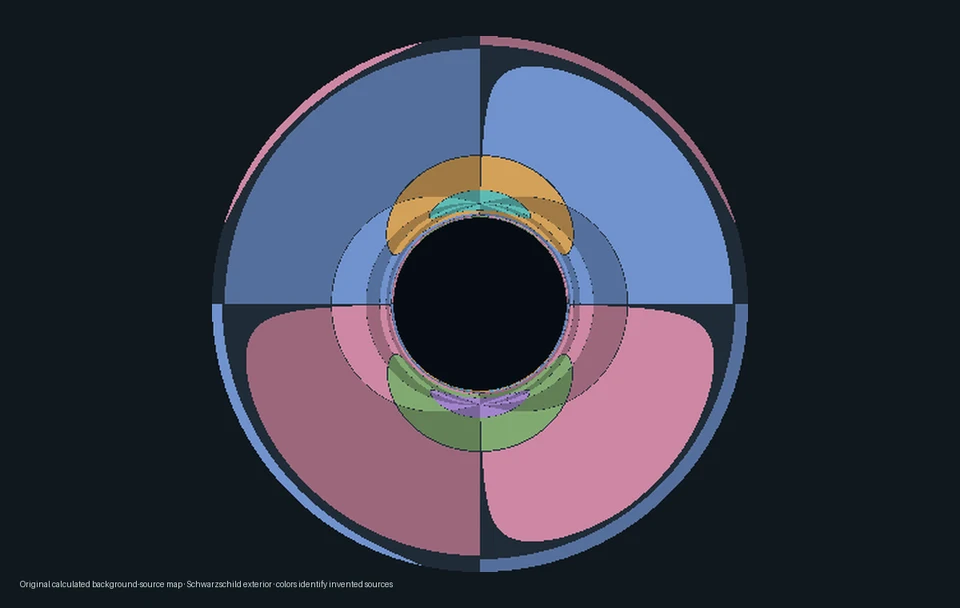 Interactive exploration
Inspect the real EHT observation, then choose a direction in a calculated light map. Follow its exterior path, find its source and reveal two images of one tiny patch.
 Interactive exploration
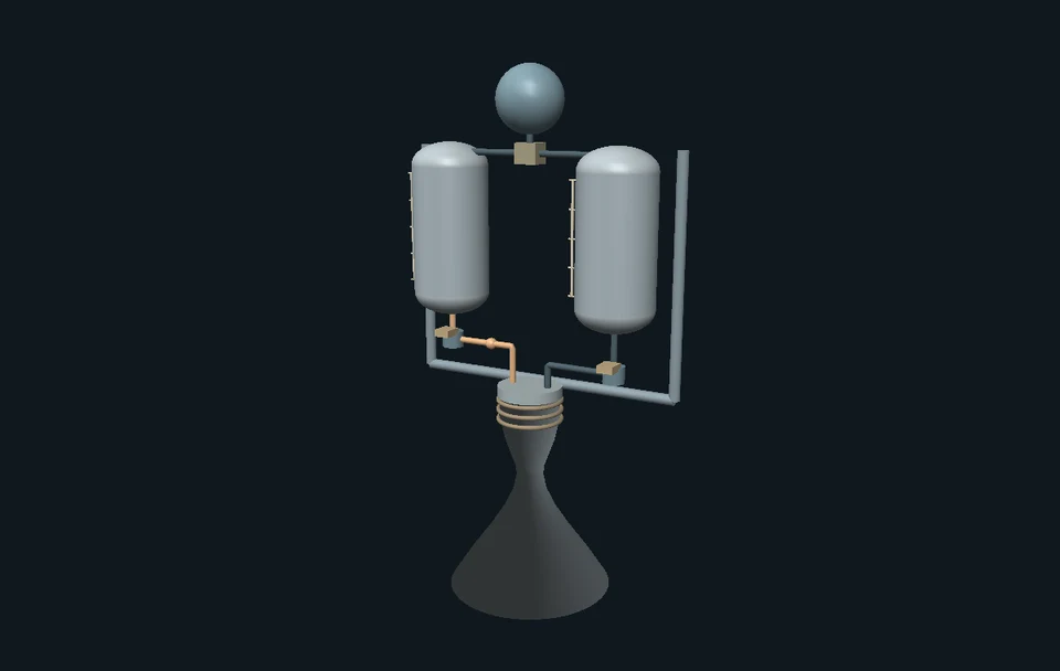
Open a generic engine, follow what it carries and keep every bit of expelled mass in the story. Change who measures the motion, balance the thrust terms and discover what staging actually changes.
 Interactive exploration
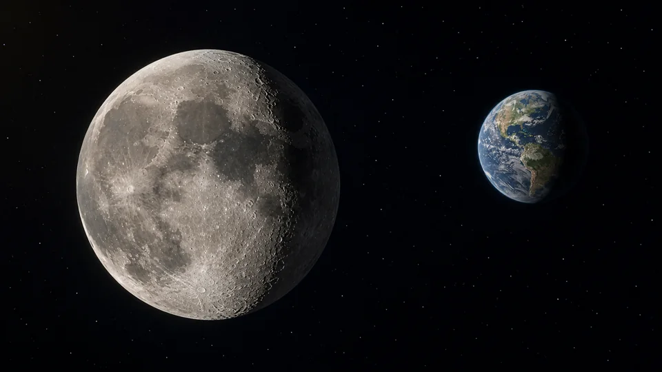
Move the Moon around Earth and compare two viewpoints at once. Make a crescent, then tilt the orbit to discover why an eclipse is a special alignment.