A fault slips; the disturbance travels
Rocks can store elastic strain energy as they deform. Slip releases some of that stored energy. The two-block illustration separates permanent offset from the small local oscillation in a passing wave.
Watch waves emerge from a buried source, pick synthetic arrivals and reveal the location one clue at a time. Test the clocks, depth and velocity assumptions—and compare the model with real recorded evidence.
Enable JavaScript to change the conditions and run the interactive experiment.
Different wave arrivals constrain distance under a model. Combining stations can locate a source, but the answer still depends on timing, geometry and what the Earth model leaves out.
One station gives you a source distance. Have you found the direction too?
One gap constrains distance under the model. Add independent station information to narrow the possible directions.
Rocks can store elastic strain energy as they deform. Slip releases some of that stored energy. The two-block illustration separates permanent offset from the small local oscillation in a passing wave.
The hypocenter is where rupture starts. The epicenter is its projection onto the surface. A buried front needs time to reach the surface; its map ring does not begin spreading from the epicenter immediately at rupture.
An ideal P wave moves material parallel to its local travel direction. S motion is perpendicular. The gold marker stays near its own equilibrium position while the disturbance moves through the medium.
A station record tells a timing story. In our authored display pulses, the first motion begins at a calculated onset. A later, larger peak is not that onset. Adjust the picks and keep their precision explicit.
Under the chosen constant speeds, a bigger S−P gap means a larger source-to-station distance. One station leaves many directions possible. At a known depth, its distance sphere becomes a circle of possible horizontal positions.
Two stations can leave two locations. A third non-collinear station can distinguish them in this exact model. If the data or model do not agree, keep that disagreement visible rather than moving circles until they meet.
A late S pick changes a gap. A station clock error can shift both phases while preserving its gap. A different assumed medium changes the interpretation. Several different depths and origins can fit three P arrivals exactly.
Real Earth structure, propagation and instruments are richer than this local model. The historic PMM recording and Loma Prieta comparison retain their original annotations. They are evidence with their own scales and limitations.
This lesson uses a flat zero-elevation surface and one isotropic solid with vP=6.2 km/s and vS=3.57 km/s. Those chosen speeds are traceable to the Canadian EPB location model described in USGS OFR82-777. Our fictional event is not a reconstruction of its New Brunswick aftershocks. The original study included elevation corrections; this model does not.
Coordinates are local kilometres: x east, y north and h positive downward. R²=(x−xᵢ)²+(y−yᵢ)²+h². A source at origin time t₀ gives P=t₀+R/vP and S=t₀+R/vS. The 3D map uses [x,−h,−y] with one common scale.
S−P=R(1/vS−1/vP). With the stated speeds, the coefficient is approximately0.118821722 s/km and R≈8.415969582 times the gap in seconds. A5.00 s gap gives42.07984791 km. It supplies a source distance, not a direction.
At known depth h, the map radius is ρ=√(R²−h²). The default source is(30,40,12) km, origin20 s; stationA is at(0,0,0). Its source distance is51.419841 km but its horizontal radius is50 km. If R<h, no exact circle exists at that depth.
After elapsed time τ, a direct spherical front has radius vτ. Its surface intersection exists only for τ≥h/v and has radius√((vτ)²−h²). At12 km, P emerges at1.935484 s and S at3.361345 s. The initial apparent ring speed is a geometric intersection effect, not a faster material wave.
With three non-collinear surface stations and exact P/S gaps, squared-range differences solve x and y; R²−ρ² gives h². Selecting h≥0 chooses the below-plane branch. Three P times alone leave four unknowns(x,y,h,t₀), and the reference examples give distinct depth/origin combinations with the same P arrivals.
For a candidate source, t₀*=Σwⱼ(tⱼ−Tⱼ)/Σwⱼ. RMS=√[Σwⱼ(tⱼ−t₀*−Tⱼ)²/Σwⱼ]. The examples use equal positive weights on six arrivals. RMS is in seconds; it depends on the model and picks. Small residuals do not prove spatial accuracy or predict another event.
Authored P and S reading bounds of±0.05 and±0.10 s give a worst-case gap bound±0.15 s and source-range bound±1.262395437 km. At a fixed depth these become annuli. The continuous overlap is not a rectangle or a statistical confidence interval. Separate coordinate extrema are computed from boundary intersections and circle extrema.
The map’s filled cells sample the band overlap at1 km cell centers; absence of a sampled cell is not proof that a smaller overlap is absent. Rounded0.01 s paper times instead have±0.005 s time-rounding bounds and±0.01 s worst-case gap rounding. That is different from the larger reading-bound exercise.
Generation controls recompute synthetic records after moving the fictional source or station geometry. The reference audit freezes its original observations before changing a pick, clock or assumed speed. The proposed fourth station compares two fixed P-only source candidates; it does not create a new earthquake or forecast.
The local marker illustration uses a chosen sinusoid and envelope. Its direction respects the inclined ray, but its frequency, amplitude, repeated timing and display length are authored. Real paths include refraction, reflection, conversions, surface waves, attenuation, radiation patterns and finite rupture. Propagating shear S waves do not traverse a liquid; no interface solver is implemented here.
Magnitude estimates event size using a specified method. Shaking intensity varies with location. Propagation, local geology, radiation and instruments affect recordings. A gain control on an arbitrary synthetic pulse cannot establish a real magnitude or damage level.
Seismic stations contribute observations to a common inference. Their geometry and clocks matter alongside the travel-time model. An added station is useful when its evidence distinguishes plausible alternatives.
The fixed observation audit shows why matching some data can leave an assumption unresolved. A P-only fit can hide depth/origin tradeoffs; a common clock offset can preserve a same-station gap.
Historic recordings connect one event to different local responses. This helps explain why a location or magnitude alone does not describe everyone’s shaking.
Use1 cm=10 km. Draw east x from−10 to110 km and north y from−60 to120 km. Mark A(0,0), B(100,0) and C(0,100). Both two-station candidates need room.
Use the rounded calculated P/S cards. Subtract P from S at each station. Record the units. These are authored examples, not recordings of an event near you.
Multiply each gap by8.41597 km/s to find source distance R. At known depth12 km, use the supplied table or√(R²−144) to get horizontal radius ρ.
Draw A and B circles. Their intersections are near(30,40) and(30,−40). Mark both before adding C. Drawing and rounded-card precision permit small mismatches.
Draw C’s circle and identify the compatible northern neighborhood. Write the epicenter separately from the12 km depth label. Describe why C added information.
Use the app’s separate reading-bound exercise to draw bands instead of thin circles. Record why an overlap region is not an exact point or a future-event prediction.
Which part came from the data, and which part came from the assumed speeds and depth?
A paper model activity with rounded calculated cards. No household vibration sensing, physical shaking experiment or future-earthquake interpretation is involved.
Slip releases stored strain energy; waves cause local motion Permanent fault offset and local wave oscillation are different motions.
Left and right P displacement is parallel to the local ray. Perpendicular displacement can illustrate S.
Source distance, without a unique direction The gap supplies a model-dependent source distance.
50 km ρ=√(R²−h²)=50 km in this case.
No, both satisfy those data Retain both candidates until independent information distinguishes them.
No, different depths and origins can share those P arrivals The reference table contains distinct exact P fits. Complete P/S pairs are a different information set.
Keep the data, show reading bounds and inspect assumptions Preserve observations and inspect picks, clocks, depth, speeds and uncertainty.
Local conditions and recording systems can affect the signals Event magnitude and location-dependent shaking are distinct. Calibrated information is needed for quantitative interpretation.
Lisa Wald/USGS, mechanism, recording and location sections. The lesson adds explicit buried-source and depth-plane geometry.
USGS · The science of earthquakesUSGS historical account of Reid’s elastic rebound interpretation after the1906 earthquake. The original two-pose illustration is not a quantitative rupture model.
USGS · Elastic reboundCranswick et al., USGS Open-File Report82-777, Results: EPB used a homogeneous half-space with6.2 and3.57 km/s plus elevation corrections. This lesson supplies a separate flat-surface fictional geometry.
USGS · New Brunswick reference modelUSGS description includes comparison of measured/predicted times and least-squares location. Depth and origin are inferred quantities.
USGS · Locating earthquakesComCat documentation for depth, depthError, rms and time. The lesson’s synthetic equal-weight RMS is not an official catalog uncertainty.
USGS · ComCat field definitionsLisa Wald USGS diagram explanation: P can propagate through solids/liquids; a propagating shear S wave does not cross a liquid. Linked context; image not bundled.
USGS · P and S wave pathsTauP3.2.0 documentation: PREM, depth200 km,57.4°, P566.77 s and S1028.61 s. The461.84 s difference is arithmetic from rounded documented predictions; no TauP run or measurement is claimed.
University of South Carolina · TauP TimeUSGS Teleseisms example: April23,2000 Argentina M6.9 Mw event, approximately600 km depth, origin09:27:23.1 UTC. Annotated PMM P/S times09:38:55 and09:48:25 yield570 s. Original wrapped display retained.
USGS · Seismogram examplesUSGS explanation of display conventions. The local GIF is not raw calibrated waveform data.
USGS · About seismogramsUSGS distinguishes magnitude, energy release and location-dependent shaking intensity.
USGS · Magnitude and intensityUSGS Public Domain media record:1989 M6.9 event, approximately equal station distances and bedrock/mud/sand-gravel displays. Original800×306 composite unchanged; no calibrated amplitude axis provided here.
USGS · Loma Prieta site responseUSGS-produced information generally public domain unless third-party rights are indicated. PMM source/image has no third-party credit shown; the Loma Prieta page has its own explicit Public Domain field.
USGS · Publication and media rightsUSGS distinguishes earthquake prediction from existing scientific capabilities. No future-event claim is part of this lesson.
USGS · Prediction limitsIndependent subject review is pending.
Read the sources and model assumptions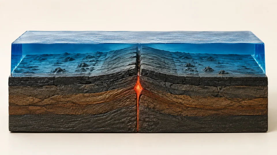 Interactive exploration
Pull a ridge apart over millions of years. Read the age and magnetic pattern left behind, then compare spreading, sliding and subduction.
 Interactive exploration
Follow water above and below the surface. Pave part of the land, change evaporation, and watch the water budget rearrange.
 Interactive exploration
Freeze two model temperatures, change infrared transfer and release time. Follow every energy route, move the accounting boundary and compare the model with real atmospheric evidence.