Move the same distance twice
Set a small sideways target for the upper plate. Keep a trial, then repeat that target over a different duration. Compare the force at each move’s endpoint, not two different final distances.
Make the same small move at different speeds, park a material-testing carriage, and watch its force change. Explore polymer networks, relaxation, creep and real research images without inventing a breaking rule.
Enable JavaScript to change the conditions and run the interactive experiment.
How a soft material responds can depend on how quickly you move it. A temporary network has more opportunity to rearrange during a slow change. In our small-shear model, the same final deformation can therefore require different forces. Fracture is a separate question that needs additional evidence.
Two moves end at the same nonzero small deformation. Must the final force match?
The faster ramp permits less relaxation while moving. Compare equal targets using retained trials.
Set a small sideways target for the upper plate. Keep a trial, then repeat that target over a different duration. Compare the force at each move’s endpoint, not two different final distances.
The plate stays at its chosen position. The force can fall while the total deformation stays fixed. This is stress relaxation: a changing response under a fixed shape condition.
The constant-load experiment imposes a small shear stress instead of fixing the plate. The deformation increases while that load stays on. This is creep.
In the ideal Maxwell model, the recoverable contribution unloads immediately while the accumulated viscous deformation remains. A real material can have additional recovery processes.
Driving the plate back forces a different motion. It can require a force in the opposite direction. That is not the same boundary condition as removing the force and allowing the material to respond.
A polymer molecule has a long backbone. Temporary connections can help form a network that rearranges while backbones remain intact. Water-rich slime contains molecules and water; it is not a single enormous molecule.
Viscoelasticity combines recoverable and dissipative aspects of material response. Say “vis-koh-ee-las-TIS-ih-tee.” The response depends on the material, conditions and time scale; the word polymer alone does not specify it.
The research images show a particular Tetra-PEG sample under increasing oscillatory shear amplitude. Separate experiments have observed fast extension and rupture in certain PVA–borate films. Neither supplies one breaking speed for every home slime.
The numerical anchor is Sato et al.’s 20 kg/mol, 60 g/L Tetra-PEG network at 25°C. Their reported Maxwell fit gives G = 4800 Pa and τ = 0.39 s. These are rounded fit parameters, not universal polymer constants.
The reported small-amplitude oscillatory sweep used strain amplitude 0.01 and angular frequency 0.01–10 rad/s. Our controlled ramps, holds and releases are model-derived transients using that fit; they are not measured pull traces from the paper.
The Maxwell model has γ = γ_elastic + γ_viscous, σ = Gγ_elastic and dγ_viscous/dt = σ/η, with η = Gτ = 1872 Pa·s. The spring and dashpot are constitutive analogies, not literal pieces inside slime.
For constant strain rate v during Δt, σ_next = σ_previous exp(−Δt/τ) + Gvτ[1 − exp(−Δt/τ)]. Signed stress is retained through reversals. Fixed-position holds set v to zero; stress then decays exponentially.
After one τ at fixed strain, the remaining ideal stress is exp(−1), about 36.8% of its starting value. It is not zero. A macroscopic network relaxation time is also not automatically one junction’s bond lifetime.
For constant stress σ₀, γ(t) = σ₀/G + σ₀t/η. At zero-load release, the ideal elastic term recovers and the viscous term remains. With 12 Pa held for 0.39 s, strain approaches 0.005 before release and becomes 0.0025 afterward.
The original uniform teaching cassette assumes area 1 cm² and gap 2 mm. Force = stress × area; displacement = strain × gap. A 1% shear is 20 µm sideways, and an ideal 48 Pa step corresponds to 0.0048 N. Enlarging motion on screen does not change these values.
For x = ωτ, G′ = Gx²/(1+x²) and G″ = Gx/(1+x²). Both equal G/2 at x = 1, where the loss modulus peaks. Angular frequency ω is in rad/s; ordinary frequency is ω/(2π) Hz.
τ divided by an experiment duration compares relaxation and imposed time scales. Strain rate multiplied by τ is a different dimensionless quantity. Neither is a probability of snapping or a universal breaking deadline.
This model can flow indefinitely under sustained load, unlike an ideal network with permanent equilibrium elasticity. Real polymer materials can require distributions of relaxation times, additional elastic contributions or nonlinear models.
An increased transient force during a quicker imposed deformation is not itself a steady shear-thickening measurement. Concentrated particle suspensions and temporary polymer networks can resist motion through different mechanisms.
Sato Figure 5 maps optical retardation in nanometers and accompanying brightness under six large strain amplitudes. The paper distinguishes nonlinear response from detected spatial heterogeneity. These images are not molecular pictures, temperature maps or observations inside our small-strain solver.
An engineer asks how long and how often a soft part is loaded, then chooses evidence for that condition. Feeling soft once does not specify long-term response.
Keep geometry, target deformation and loading history attached. Changing two of these at once does not isolate a speed effect.
A realistic-looking sample can illustrate a tested model without predicting drying, damage, ingredient effects or household product performance.
Use this activity without making or buying slime. Tear or fold two equal strips and keep another sheet for a simple grid and junction marks.
Fold loose zigzags and draw a continuous line along each strip. Place the strips side by side. Draw a few removable junction marks on the separate sheet.
Mark a start and a target one grid square away. Predict what changes if there is more time to redraw connections between moves.
Move a paper grip one square per count. Allow one junction redraw between moves. Record how many opportunities the rule allowed; do not call the paper’s stiffness a slime measurement.
Repeat the same moves, allowing five redraw counts between them. Keep the backbone line continuous. Compare the opportunities in the two invented schedules.
Explain imposed motion versus time to rearrange. The paper rule does not measure G, τ, ingredients or fracture. Return to the controlled digital trials and identify which quantity was held fixed.
How did the time you allowed change the opportunities to rearrange—and what did your paper fail to measure?
No scissors, glue, powders, borax, contact-lens solution, heating or chemical mixing is needed. If observing an already-prepared age-appropriate slime separately, follow its label with an adult, keep it on a tray, avoid faces and food, stop if it irritates, and wash hands afterward. Do not escalate pulling to force a snap.
It leaves less time for relaxation during motion Motion history competes with relaxation in this model.
Stress relaxation Position stays fixed while stress changes.
Creep Creep is time-dependent deformation under a sustained load.
An elastic part recovers; a viscous part remains The recoverable and viscous contributions are distinct.
No, material structure and conditions also matter Polymer identity alone is not a mechanical specification.
Their structures and loading need different evidence Similar large-scale observations can come from different mechanisms.
Optical retardation Read the source color scale and units: nanometers of retardation.
No, fracture and formulation need additional evidence The linear model does not solve fracture.
Table 1, Mw 20 kg/mol and 60 g/L: G 4800 Pa, τ 0.39 s. Figures 1, 2 and 5 retain specimen identity and CC BY 4.0 credit.
Sato et al. (2026) · Controlled transient networksAuthor-deposited article XML. The complete local source and exact extraction provenance are retained; this is not a raw rheometer time series.
Europe PMC · Sato primary full textFigure 1 chemistry scheme and measured network responses. CC BY 4.0; a different material from the numerical specimen.
Taniguchi & Urayama (2021) · PVA network responseSteel-ring film extension and formulation dependence. No universal household threshold is inferred; this paper’s noncommercial images were not redistributed.
Deleurence et al. (2018) · Transient hydrogel filmsIndependent binding and network-response comparisons show connectivity matters.
Katashima et al. (2022) · Network connectivityEquations independently implemented with original graphics; noncommercial course diagrams were not copied.
MIT · Roylance, Engineering ViscoelasticityAn individual polymer molecule and a material composed of molecules are different levels of description.
IUPAC · Macromolecule definitionDistinguishes viscoelastic response and time-dependent deformation under load.
IUPAC · Polymer terminologySilica-suspension experiments on frictional and hydrodynamic contributions; their numerical results are not used as cornstarch measurements.
NIST / Royer et al. (2016) · Shear-thickening suspensionsPrimary research on shear thickening and jamming, separate from the transient polymer-network lesson.
Fall et al. · Cornstarch suspensionsSource-owner precautions; we do not reproduce its chemical recipe or require a new preparation.
American Chemical Society · Connect with SlimeSupports using the paper alternative and avoiding added household chemicals.
National Capital Poison Center · BoratesIndependent subject review is pending.
Read the sources and model assumptions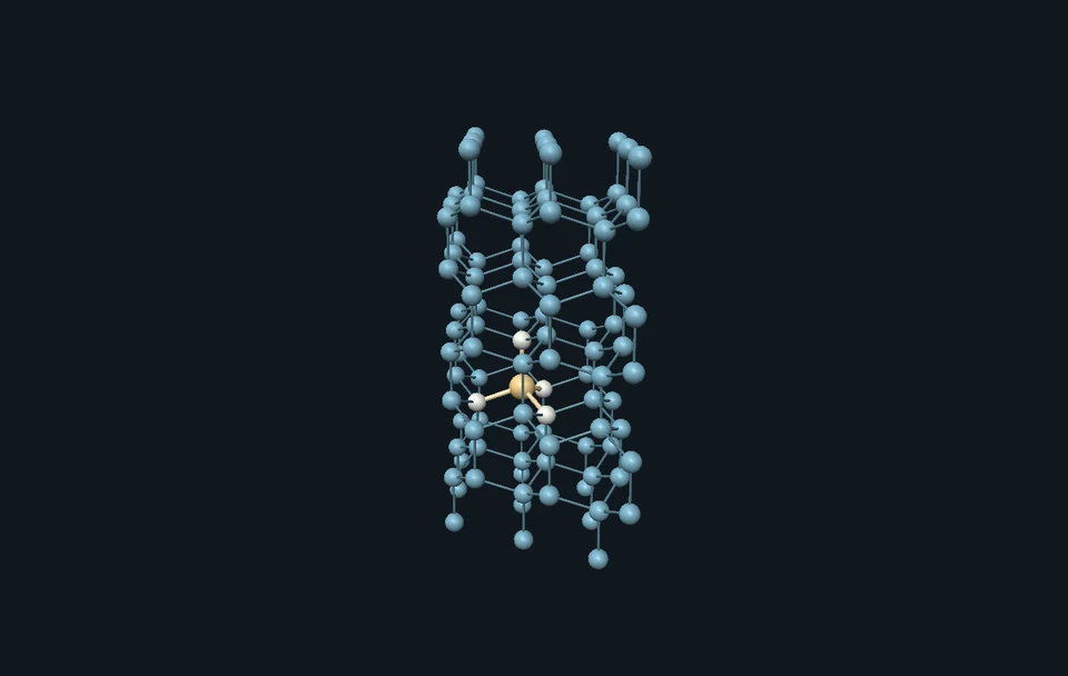 Interactive exploration
Give water an energy budget. Watch its temperature and phase masses, catch a melting plateau, compare two starting states and inspect an open ice structure.
 Interactive exploration
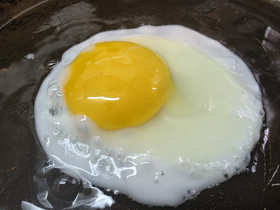
Tilt a plate, press a sample, and tug the connections that help a cooked egg hold together. Inspect a real ovalbumin structure, compare source-defined laboratory holds, and uncover what an experimental photograph actually shows.
 Interactive exploration
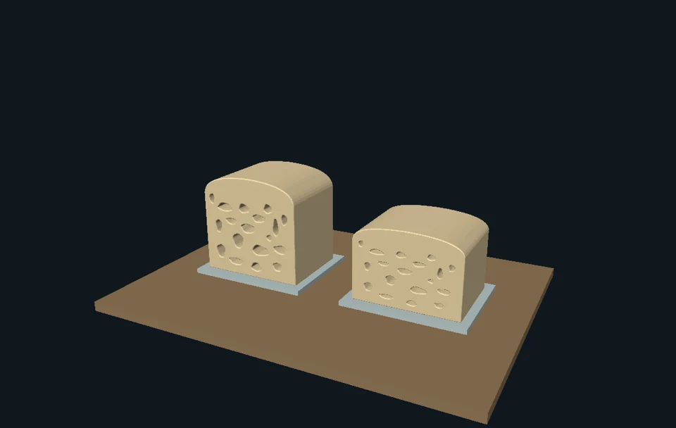
Slice into two teaching doughs, follow gas as it is made, kept or lost, and discover the microbes and chemistry behind rising bread. Inspect real microscopy and a yeast enzyme.