Start with one exact question
A fictional print shop asks whether a dot’s center is inside a circular guide. Its decorative A/B batch mark is not part of that geometric rule. The dot’s visible size is not what is classified.
Train a real classifier on editable inspection cards. Reveal a confident mistake, repair a misleading shortcut, and freeze your model before opening its reserved test.
Enable JavaScript to change the conditions and run the interactive experiment.
Matching examples is not the same as learning the intended rule. What a model can see, which annotations it receives, and how you evaluate it all shape what a good-looking score really means.
A model matches all 25 training annotations. What can you conclude?
Training classifications can all be correct while loss remains nonzero and new cards reveal confident mistakes.
A fictional print shop asks whether a dot’s center is inside a circular guide. Its decorative A/B batch mark is not part of that geometric rule. The dot’s visible size is not what is classified.
The model receives numeric coordinates and the selected fixed features. It does not read pixels. A straight model sees x and y; a curved model also receives x²+y². The designer supplies this useful representation, while training learns its weights.
Every training update computes prediction errors from supplied annotations and adjusts all weights together. The score maps, weight table and loss curves use the same recorded weight snapshot. Playback reveals real optimization steps.
A flexible model can fit the deliberately wrong outside-card annotation. It may then call a nearby outside dot inside with a high score. Compare the supplied label with the separately defined guide, then correct and refit.
The correlated-batch preset puts inside examples in A and outside examples in B. A batch-only model can look perfect on familiar marks. Reverse only the marks and inspect its predictions without changing positions or weights.
Remove the batch feature or supply both marked versions at each training location. These paired cards share lineages; they are not independent measurements. Verify the repair on appropriate probes rather than assuming more examples always help.
Use validation for choices, freeze the currently inspected weights and threshold, then open the reserved envelope. Once answers have influenced your choices, placing those same answers back in an envelope cannot make them unseen again.
Each dot has integer coordinates u,v from −1000 to 1000; x=u/1000 and y=v/1000. The answer is inside when u²+v²≤490000, including the boundary. The guide radius is 0.7 and both map axes have equal scale. This is invented teaching data, not a production benchmark.
The feature vector contains only selected position calculations and possibly a stored visible batch mark. Guide answers are evaluator metadata. Training uses the annotations supplied on training cards, including intentionally wrong ones.
The score is σ(w·f), where σ(z)=1/(1+exp(−z)). The main feature choices have 3, 4 or 29 weights. Flexible features add 25 fixed Gaussian bumps centered on a declared grid with width 0.2. These centers and widths are not learned hidden neurons or an infinite kernel.
Training minimizes mean binary log loss plus λ/2 times the sum of squared non-intercept weights. The intercept is unpenalized. The workbench reports data loss, penalty and total objective separately. Natural logarithms give nats per example.
The gradient averages (score−annotation) times each feature, then adds the non-intercept penalty gradient. All coordinates update from the old weight vector. The conservative step η=1/B uses B=Σ||f||²/(4n)+λ, an upper bound derived from σ(1−σ)≤1/4. Validation and reserved labels are absent.
Weights start at zero and at most 5000 updates are recorded. Editing examples, features or λ starts a fresh fit. In unregularized separable logistic regression, weights may continue growing as loss approaches zero. A finite update budget does not promise exact convergence or zero loss.
On the symmetric clean grid, the straight model settles at a constant inside score 9/25=0.36. A straight boundary cannot enclose the center while excluding the surrounding outside examples. Running more identical updates cannot add a missing representation.
On the fixed noisy flexible example, λ=0 gives 35/36 validation classifications and mean loss about 0.106845; λ=0.02 gives 36/36 but loss about 0.345015. Regularization improves one criterion here while worsening another. Neither is a universal ranking of model quality.
A fitted score near 0.96 can be wrong on the deliberately noisy fixture. Calibration is about the relationship between predicted probabilities and observed outcomes across suitable data; a confident single prediction does not establish it.
Classify inside when the unrounded score is at least the threshold. Raising the threshold cannot increase true-positive or false-positive counts on fixed data. It leaves weights, scores and log loss unchanged. Exact ties count as inside.
Inside is the positive class. TP finds an inside center, FP calls an outside center inside, FN misses an inside center, and TN rejects an outside center. Accuracy divides all correct predictions by all cards; precision divides TP by inside predictions; recall divides TP by actual inside cards. A zero denominator is undefined.
Training fits weights; validation guides choices. A reserved set evaluates a frozen choice. Using reserved scores to tune settings compromises their untouched role even when none of those rows enters a gradient. The exposure marker persists locally.
The 64 reserved integer-grid positions use a documented 32-bit LCG with coordinate seed 48 and independent mark seed 49, rejecting original training/validation coordinates and duplicates. Their balanced class count happens for this seed; the generator does not enforce it. The code and answers remain inspectable, so this is not a secure exam.
Validation and reserved records stay fixed when training is edited. A shared coordinate or lineage is flagged. Changing an ID does not make a copy independent. The original validation grid is deliberately designed, rather than a representative random sample of a factory population.
A pre-existing decoration can support a misleading shortcut without being a future answer leak. Reversing marks changes the input distribution while the geometric rule stays fixed. For a batch-only predictor, the target relationship conditional on its restricted input changes. An inspection-answer field created afterward is excluded for a different reason: it is unavailable at prediction time.
If a shop changes its guide radius from 0.7 to 0.5, the same position (0.6,0) changes answer. That is a new target rule, not just a different mix of positions. Our interactive workbench keeps radius 0.7 fixed; the old weights would not automatically adapt to a new specification.
Write the prediction question, when each input is available, what the labels mean and which data influenced selection. A percentage without those details can conceal a different task.
Inspect individual errors and change one factor at a time. A missing representation, wrong annotation, changed input distribution and leaked answer require different explanations.
Ask whether a reported result used a frozen choice on appropriate new examples. This toy exercise does not certify any real product, but it makes the evaluation questions concrete.
Training: inside dots (0,0), (0.4,0), (0,0.4), (−0.4,−0.4), all marked A. Outside dots (0.8,0), (0,−0.8), (−0.8,0.8), (0.8,0.8), all marked B. Keep other pockets closed.
Open only training answers. Write a rule another person could apply. A means inside fits all eight, but the examples alone have not established that decoration is the intended mechanism.
Predict (0.3,0.3) B and (−0.5,0) B as inside; (0.7,0.4) A and (−0.7,−0.4) A as outside. Reveal only after writing predictions. This deliberately reversed-mark set is a stress probe.
Use the validation mistakes to revise. A helper can now reveal x²+y²≤0.49 or provide more training cards. Write exactly what informed your frozen rule before looking at final answers.
Final key: (0.2,−0.5) A inside; (−0.6,0.1) B inside; (0.8,−0.2) A outside; (−0.6,−0.6) B outside. A helper should fold the key under before the learner starts. Count all four outcomes.
Swap marks on a known card and explain what your rule uses. If you revise after seeing final answers, label that rule revised after test. Reading this printed answer key also counts as exposure.
Which information changed your rule, and which answers were still unseen?
This is a paper process analogy, not a human-versus-AI benchmark. Four final cards do not establish production accuracy. No personal data, account, camera or powered equipment is required.
Is the dot center inside the guide? The target is defined by geometry. Appearance and value are neither labeled nor measured.
Its chosen features cannot express that enclosure On this symmetric grid its constant optimum is 0.36. Optimization cannot turn the selected family into a circular boundary.
The model can extend a wrong annotation into a confident error The geometric answer is independent of the fitted score. Correcting the supplied annotation and refitting tests this explanation.
This model depends on the mark at this location Position and weights stayed fixed. The controlled mark intervention exposes this predictor’s dependence.
No, those answers influenced selection Information can enter through model choices as well as gradient updates.
1/2 and 1/2 Two of four predictions are correct; one of two actual inside cards is found. The denominators differ.
Scores and log loss Thresholding changes the decision rule, not the fitted scores or their probability loss.
The target specification This hypothetical new rule differs from changing where cards occur while retaining the answer rule.
Stanford CS229 notes, Chapters 2 and 5. Feature bank, data, penalty convention and step bound in this lesson are explicitly authored choices.
Stanford CS229 · main notesMean binary cross-entropy and regularization concepts. Our scalar values and experiments come from the declared synthetic model.
Google MLCC · loss and regularizationSeparate fitting, selection and final evaluation. A fixed designed grid does not become representative of production merely by being held out.
Google MLCC · dividing datasetsData unavailable at inference or evaluation information must not leak into fitting. Our feature coordinates and centers are fixed in advance.
scikit-learn developers · common pitfallsCawley and Talbot, JMLR 2010. Supports the exposed-test state even when test rows never enter a gradient.
Cawley & Talbot · model-selection biasGeirhos and colleagues, 2020. This lesson’s simple logistic batch-mark analogy is an original example, not a reproduction of their neural-network results.
Geirhos et al. · shortcut learningGuo and colleagues, ICML 2017. A fitted probability estimate is not automatically an observed correctness frequency.
Guo et al. · calibrationInside is our positive class; exact ties count as inside and undefined denominators are retained explicitly.
Google MLCC · classification thresholdsKoh and colleagues, ICML 2021. No WILDS datasets, images or performance numbers are imported into this synthetic workbench.
Koh et al. · WILDSIndependent subject review is pending.
Read the sources and model assumptions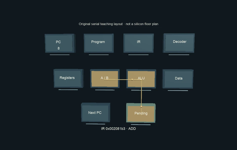 Interactive exploration
Write a tiny real assembly program, watch values move through a processor’s logical parts, and stop at the instant an answer becomes stored state.
 Interactive exploration
Inspect a connected CMOS cutaway, build a channel, find a circuit’s operating point and follow the charge and energy behind a changing bit.
 Interactive exploration
Flip real input bits on a little calculator. Build a result from simple rules, and follow a carry as it crosses four columns.