Investigate a virtual garden. Change who receives an assignment card, uncover a hidden starting difference, run fair trials and discover why a pattern alone cannot settle what caused it.
Enable JavaScript to change the conditions and run the interactive experiment.
Understand it
Make a prediction from the pattern
In the opening recipe, 30 of 50 baseline-only plots meet a target, compared with 25 of 50 extra-water plots. Those are exact constructed proportions. Decide what the chart establishes before revealing two different response stories.
Follow the assignment card
Open the garden. W0 means baseline care; W1 means an extra-watering assignment. The card is a variable you can change. Each bed keeps its own stored baseline category and response digit when you change assignment.
Reveal a harder starting point
The default existing policy gives extra-water cards to drier plots more often. Those plots also have a harder baseline. Open the soil layer without redrawing the city. This common cause can make a beneficial rule look harmful in the pooled comparison.
Replace the assignment rule
Shuffle equal numbers of W0 and W1 cards independently of dryness. The baseline-to-assignment link is removed. Dryness still affects success, and the stipulated response effect still operates.
Compare filtering with setting
Showing only plots that already have W1 retains a selected subset. Setting every plot to W1 retains the whole original cohort and replaces assignment. Compare the row counts and baseline composition side by side.
Keep the denominators
Split the comparison into dry and less-dry categories, then average each arm’s category rates using the same 50/50 target mix. An empty sample cell has no rate; this calculation stays unavailable rather than guessing a value.
Repeat, then explain the variation
Generate fresh cities and independently shuffle their assignments. Small estimates vary even when the model effect is known. Keep all repetitions, compare them with the exact sampling distribution, and distinguish sampling more plots from running more repetitions.
Look closer at the science
Correlation and risk difference are different summaries
For binary W and Y, the workbench can calculate their correlation and the difference between success rates in the two observed arms. Neither summary alone specifies the effect of replacing an assignment mechanism. A zero-variance variable makes correlation undefined.
The original structural causal model
C marks baseline dry-soil category, W marks the assignment, and Y marks a single binary endpoint. Independent population digits RC, RW and RY are uniform on 0 through 9. In A, C=1[RC<5], W=1[RW<5+k(2C−1)], and Y=1[RY<7−5C+tW]. These are authored mathematical rules, not measured plant biology.
Bounded rules need no probability clipping
A permits t=0,1,2 and k=0,1,2,3,4. The within-category benefit is t/10; k controls how strongly the existing policy favors dry plots. Assignment probabilities remain between 0.1 and 0.9, so both assignments are possible in both categories in the population.
An observational reversal
With t=2,k=3, the extra-water population is 80% dry while the baseline-only population is 20% dry. Both within-category intervention differences are +20 percentage points, yet observed rates are 50% versus 60%. This reversal is related to Simpson’s paradox; the causal graph determines which comparison answers the intervention question.
Exactly the same W/Y law, opposite causal effects
Rulebook B retains the default assignment policy but uses Y=1[RY<6−W], with no direct C-to-Y effect. Both worlds have joint probabilities W0Y0=.20, W0Y1=.30, W1Y0=.25, W1Y1=.25. A has intervention risks .45 and .65; B has .60 and .50. These are equal population observational laws, not a claim that independent finite samples have identical counts.
Identification is not precision
More observations of only W and Y estimate their common distribution more precisely without selecting between A and B. Measuring the baseline variable or performing the stated intervention can distinguish these particular worlds in principle. This does not mean observation is useless: appropriate assumptions, measured variables and study design can support causal identification.
Conditioning versus intervention
P(Y|W=1) refers to the existing W1 group. P(Y|do(W=1)) replaces the assignment equation and keeps the full population’s background distribution. The simulator implements the latter by setting W while retaining each stored C and RY. It does not manipulate Y directly to force a preferred answer.
The declared graph justifies this adjustment
In default A, C causes both W and Y, creating a back-door path. Standardizing category-specific means to a common 50/50 city composition recovers the intervention contrast at the population level. This depends on the stipulated sufficient baseline variable and positivity. It is not permission to adjust for every variable in an arbitrary dataset.
A population possibility is not a sample observation
Positive assignment probability in each category does not guarantee all cells appear in a sample of 20. The default observational cohort has no dry baseline-only plot. Its sample cell mean and cell-mean standardized difference are unavailable. Zero rows are not a 0% success rate.
Random allocation does not guarantee a balanced realized sample
The balanced shuffle assigns exactly N/2 plots to each arm. In the reproducible default 20-plot city, randomized arms contain 6 dry plots versus 2. That chance imbalance does not prove the randomizer is broken. Outcome comparison must respect the planned allocation and sampling procedure.
Random assignment and random sampling do different jobs
Assignment governs which response is observed for each sampled unit. Sampling governs which units enter the study. Random assignment alone does not establish representativeness, transportability, absence of missing outcomes or adherence to the assigned action.
One unit, two stipulated response boxes
The oracle computes Y(0) and Y(1) using the same unit’s C and RY. This coupling defines individual response types inside the simulator. A real experiment ordinarily observes one outcome under one assignment in the same circumstances. An average effect by itself does not identify each individual’s response.
Three quantities deserve three labels
The known population effect averages over the declared probability law. The finite-cohort oracle averages paired Y(1)−Y(0) over the stored plots. The observed arm-rate difference compares different realized groups. These can differ in a finite sample without any calculation being wrong.
A zero effect can have a nonzero estimate
At t=0 in A, every unit’s paired outcomes agree, so both population and finite-cohort causal effects are zero. Different units still fall into the two randomized arms; a realized comparison can be nonzero. Under the confounded existing policy at k=3, the population observational contrast remains −30 percentage points.
An exact fresh-city distribution
Under default A, fresh randomized arm successes are independent Binomial(n,.65) and Binomial(n,.45), where n=N/2. Their difference divided by n has mean .20 and variance .475/n. The chart calculates every possible mass by convolution. The shown central sampling range uses discrete 2.5% and 97.5% quantiles; its actual included mass need not be exactly 95%.
A surprising result under a known positive effect
For 20 fresh plots, the standard deviation is about 21.79 percentage points and a zero or negative estimate occurs about 24.35% of the time. At 400 plots, standard deviation falls to about 4.87 points. Those are probabilities under a specified positive-effect model, not p-values or probabilities that the effect is zero.
A fixed paper deck has a different uncertainty law
The 20-card activity contains 9 always-success, 4 helped and 7 never-success cards under default A. Exactly 184,756 balanced assignments are possible. Their mean difference is .20 and probability of a nonpositive difference is about .23107. This differs from the fresh-city value .24353 because the response-type composition is fixed.
Intervals need a named target
The optional Wilson intervals estimate individual binomial arm rates under their sampling assumptions. They are not an interval for the difference, and overlap is not a specified difference test. Approximate 95% confidence describes repeated coverage of a method, not a 95% posterior probability attached to one fixed unknown rate.
Reproducible does not mean observed in nature
The versioned SHA-256/rejection generator uses seed, cohort, unit ID, variable stream and draw index. An independent Fisher–Yates shuffle supplies balanced assignments. Filters and reveal controls leave the data unchanged. Changing sample size rebuilds that size’s allocation; it is not appending plots with all former cards guaranteed unchanged.
Sources and model limits
- Every city, digit, coefficient and outcome here is synthetic. No actual gardening, health or policy effectiveness is inferred.
- The endpoint is binary. Geometry and card motion are an inspection sequence, not a continuous growth model, time scale or calibrated water dose.
- No runoff, interference between units, clustering, missingness, measurement error or nonadherence is represented.
- The graph is stipulated, not learned from a correlation coefficient or automatically identified from arbitrary uploaded data.
- Standardization is justified for the declared baseline variable and target mix; sample empty cells remain unavailable.
- Fresh-city sampling and balanced reassignment of a fixed paper deck have separately calculated uncertainty laws.
- Simulator-only paired truth is not information a real randomized trial ordinarily provides for every unit.
- Source research and numerical verification do not certify classroom comprehension, specialist review, accessibility or device/video-export behavior.
Structural equations and intervention assumptions
Pearl’s 1995 primary paper, especially structural interpretation and causal diagrams. The garden coefficients and diagrams are original.
Pearl · Causal diagrams for empirical researchAssociation, intervention, adjustment and counterfactuals
Pearl’s 2009 overview, sections 2.1, 3.2.1, 3.3.1 and 3.4. Defines the methodological distinctions used here; it does not validate the invented gardening probabilities.
Pearl · Causal inference in statisticsConfounding and assignment mechanisms
Stark’s UC Berkeley course text distinguishes classification and observation from assigning a treatment.
Stark · Does treatment have an effect?Completely randomized allocation and paper-label procedure
NIST/SEMATECH section 5.3.3.1. Supports randomized design, not guaranteed realized baseline equality.
NIST · Completely randomized designsFixed-ticket randomization and scope of inference
Stark’s Stat 240 chapter 3. Motivates keeping fixed-card allocation uncertainty separate from fresh-population sampling.
Stark · Randomization modelsFresh-city binomial probability masses and variance
NIST/SEMATECH binomial distribution formulas. All chosen probabilities and numerical data belong to our synthetic rulebook.
NIST · Binomial distributionOptional individual rate intervals
NIST’s Wilson formula. We do not use overlap of separate intervals as a treatment-difference test.
NIST · Confidence intervals for a proportionRepeated-use interpretation of confidence
NIST explains coverage interpretation. Its mean-specific interval formula is not substituted for the binary Wilson calculation here.
NIST · Interpreting confidence limitsCorrect conditional interpretation and complete reporting
ASA’s 2016 statement, six principles. A p-value is not the probability a hypothesis is true; this lesson’s model sampling probabilities are not p-values.
ASA · Statement on statistical significance and p-valuesIndependent subject review is pending.