Look before the reveal
The two center squares may look different, similar, or somewhere in between. Keep your own observation. It is not a test of attention or a puzzle with a required visual experience.
Become a color detective. Move the surroundings, uncover the samples, and inspect the actual pixels. Then put a simple explanation to a harder test.
Enable JavaScript to change the conditions and run the interactive experiment.
A color is seen in a scene. Changing its surroundings can change its appearance while the specified center pixels stay the same. This kind of contextual effect is called simultaneous brightness contrast. Knowing the numbers need not remove the effect—and not noticing a difference is an acceptable observation.
How could you check the surroundings without changing two things at once?
The isolation control keeps the targets fixed while changing their context. Your appearance report and the pixel check answer different questions.
The two center squares may look different, similar, or somewhere in between. Keep your own observation. It is not a test of attention or a puzzle with a required visual experience.
Swap the surrounding fields while leaving both center patches in place. We repaint only the context. An experiment is more informative when its changing and fixed parts are clear.
The neutral cover leaves two cutouts for the original center patches. At full coverage, both have the same surrounding gray. This is an isolation control. The joining strip offers another comparison, but also changes grouping.
Our pixel lens reads the actual canvas image buffer. It can inspect a center, a surround or an edge. The full check counts every pixel inside both target rectangles, including its opacity.
Simultaneous brightness contrast describes a shift in appearance in relation to nearby regions. It names a phenomenon; it does not by itself specify every optical or neural mechanism involved.
Perhaps appearance depends only on the average lightness around a patch’s border. We make that proposal precise, then try a striped display associated with White’s effect. A rule that helps with one example can fail with another.
Researchers vary nearby and more remote regions separately. Spatial arrangement, scale and relationships matter. One informal screen demonstration cannot locate the effect in a particular part of the visual system.
Check a paint sample in its intended context. Inspect actual pixel values when editing an image. When explaining a chart, keep the colors, their surroundings and the viewer’s task in mind.
RGB is a digital specification. Luminance is a physical photometric quantity, measured in candelas per square meter (cd/m²). Brightness describes visual appearance. The app measures its image buffer, not the emitted light of your screen or your experience.
In color science, lightness is a relative appearance judgment involving a similarly illuminated area regarded as white. CSS HSL “lightness” is a color-coordinate parameter, not a calibrated measurement of that perceptual quantity.
The equality fixture is an 800 × 360 opaque sRGB raster. Each square contains 12,544 pixels, all RGBA(128,128,128,255). Baseline surrounds are codes 32 and 224. The full neutral mask uses 176. Integer source rectangles avoid edge ambiguity in the exact check.
For a channel c = code/255, use c/12.92 at c ≤ 0.04045, otherwise ((c + 0.055)/1.055)^2.4. Gray codes 32, 128 and 224 give normalized linear-light values 0.01444384, 0.21586050 and 0.74540421. These are not measured cd/m² or perceived-brightness scores.
Our original stripe targets are 40 × 136 pixels. Short ends contact 80 units of aligned bars; long sides contact 272 units of side bars. The candidate rule subtracts their length-weighted linear-light mean from the target level. It is auditable arithmetic, not a biological simulation.
Blakeslee, Padmanabhan and McCourt (2016) manipulated aligned and flanking bars independently. The research challenges a universal explanation based only on total light/dark border contact. Our original display is informed by that phenomenon, not a calibrated replication or a guarantee of each viewer’s report.
Blakeslee and McCourt (2023) kept target luminance at 64 cd/m², independently changed ring width/luminance and remote background, and measured matching judgments. Four observers used a calibrated display. The shown group graph uses mean matching luminance with ±1 standard error of the mean; it is not a percentile chart.
That study’s target radius was 0.5° of visual angle. Ring widths ranged from 0.1° to 24.5°; the largest outer radius was 25°. A browser pixel has no universal angular size. Copying 64 cd/m² into RGB code 64 would confuse two different quantities.
Sinha and colleagues (2020) used special experimental displays and observations after sight-restoring treatment to constrain explanations of brightness contrast. Their results argue against treating learned scene interpretation as the only cause. Our page does not reproduce those procedures or settle one exclusive neural pathway.
Troscianko and Osorio (2023) tested an efficient-coding and spatial-filtering account of color appearance. Their cube figure places an input stimulus above the model’s transformed image. A successful transformation is not a photograph of a thought, and our border arithmetic is not their SBL model.
Color management, local dimming, nonuniform output, viewing angle, room light and glare can affect the viewing condition. A screenshot checks part of an image pipeline; a physical light measurement requires suitable instrumentation. The same source numbers do not establish identical photons at the eye.
If you do not see an effect, keep that result. There is no score, timing target, age norm or attention diagnosis here. The lesson remains useful through the numeric controls, explicit hypothesis and source evidence.
Place the same sample beside the surrounding colors you plan to use. Keep an isolated reference so that changing context is visible.
Distinguish what a region looks like from what its pixels specify. Numeric inspection answers a different question from a viewing report.
Write down a rule’s prediction before choosing a second example. A counterexample can improve the explanation rather than end the investigation.
Put the light and dark papers side by side. Lay one continuous gray strip across their meeting edge. Record similar, different or not sure for its ends.
Predict what might happen. Exchange the papers beneath the strip while trying to keep the strip and lighting fixed. Record what you actually notice.
Put the same strip on the neutral sheet. Compare its ends. Did the material change, or did its context change?
If comfortable, return to the original arrangement once. Name the variable changed and the material kept. There is no required visual answer.
Look for uneven light, raised-paper shadows, texture, printing or viewing angle. One piece controls material identity better than two scraps, but does not prove perfectly uniform light or reflectance.
Can you change the setting while keeping the same piece of paper?
Use ordinary comfortable light and look normally. No bright lamps, staring, blindfolds or eye pressure. An adult can prepare a strip; no cutting tool is needed for the activity. Keep a weak or absent effect as a valid observation.
The specified center colors The fixed variable is the digital center color.
Keep both centers on one neutral surround Remove the surround difference while preserving the targets.
The sampled image-buffer values It reads the canvas buffer, not a biological or physical light measurement.
Revise or limit the rule and test more evidence A single success does not establish a universal model.
Nothing diagnostic from this observation This is an informal display experiment with no validated personal score.
A computational model’s transformed image The panel is a model output with assumptions and limits.
Digital code and luminance are different quantities Code values alone do not reproduce a calibrated light output.
Knowledge and appearance can differ Knowing a fact need not erase a contextual visual effect.
2023 primary study; four observers, calibrated display, constant 64 cd/m² targets. Original Figures 1 and 3 reused with CC BY 4.0 credit.
Blakeslee & McCourt · 20232016 primary study of White’s effect. We author our own geometry; no source figures are redistributed.
Blakeslee, Padmanabhan & McCourt · 2016Special displays and sight-restoration observations; these procedures are not reproduced in this lesson.
Sinha et al. · 2020Input and SBL-model transformation, original Figure 5. CC BY 4.0. Not a neural recording or our pixel-equality reference.
Troscianko & Osorio · 2023Perceptual attribute, distinct from an image code or physical meter reading.
CIE · BrightnessRelative appearance definition, not CSS HSL coordinate arithmetic.
CIE · LightnessPhotometric quantity with cd/m² units; cannot be inferred from a code alone.
CIE · LuminanceExact color-space arithmetic used in the explicit hypothesis. No personal brightness prediction is derived.
W3C · CSS Color 4Local unaltered figures, source XML, hashes, authors and CC BY 4.0 attribution.
Asset provenanceIndependent subject review is pending.
Read the sources and model assumptions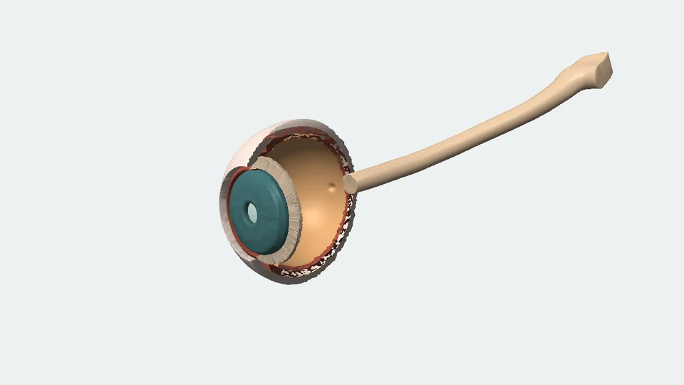 Interactive exploration
Open a sourced 3D eye, move a target nearer, and catch the moment its light comes together. Then discover why a smaller pupil is different from better focus.
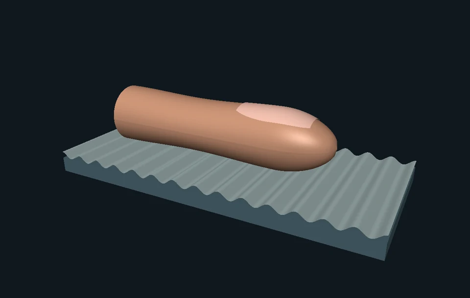 Interactive exploration
Slide a texture beneath a finger. See the contact change, compare a moving touch with a steady one, and zoom from skin to a real sensing protein. Discover how touch differs from pain.
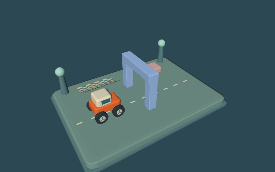 Interactive exploration
Drive an original little rover behind an arch, turn the camera, and open one pixel of the actual picture. Discover which triangle wins, where its color comes from, and what changes when you add more samples.